4.1 Real Velocity Measuring Device (RVMD)
From the preceding sections one can conclude that a RVMD (Real Velocity Measuring Device) concept is feasible. My RVMD concept is already described in more detail in my USPTO patent text (2006) but is reviewed here briefly. In my patent text different possible RVMD builds are introduced which either use no mirrors or either one to two mirrors. Mirrors are used to reflect the photons, being emitted by the photon source, in a controlled manner in order to increase the trajectory length of the photons and thus increase the magnitude of the signal shift (see e.g. the type of signal shift MF, illustrated in Figure 10) (then shift of photon at a detector). A full analysis of a three dimensional RVMD is not presented here. In that respect some more details can be found in my Elsevier publication Etienne Brauns, “On the concept and potential applications of a photons based device, measuring the velocity vector of an object, moving at high speed in space“, Results in Optics, 10 (2023) 100349, https://doi.org/10.1016/j.rio.2023.100349
To somewhat demonstrate here the basics of my RVMD concept, Figure 33 is shown.
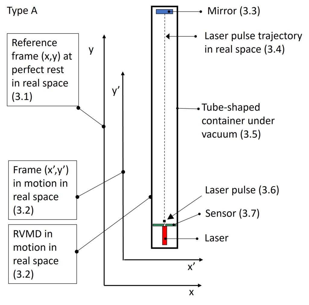
In Figure 33 a tube-like container under vacuum holds a laser (photon source), a sensor and a mirror. The laser source is geometrically mounted perfectly in a way that the laser points exactly in a perpendicular direction towards the plane of the mirror. The mirror’s plane is thus perfectly perpendicular to the y-axis. The sensor allows to locate/measure the location of the arriving photon and therefore also the signal shift which is caused by the real velocity of the RVMD in the x-direction.
It should be remarked that if the RVMD travels in the:
- right-handed x-direction at a specific velocity, the signal shift at the sensor is at the left-handed side of the sensor
- left-handed x-direction at a specific velocity, the signal shift at the sensor is at the right-handed side of the sensor
It is therefore clear that, when the x-location (x-value) of arrival of the photons at the sensor is exactly the same as the x-emission location (x-value) of the photons from the laser, such means that the RVMD device shows no signal shift at the sensor, meaning that the RVMD must be at perfect rest in the x-direction. Thus having a scalar value of the real velocity vector in the x-direction equal to zero (simply no velocity to the left nor to the right which can only be equal to perfect rest in the x-direction). The device thus enables the measurement of real velocity in one direction in real space.
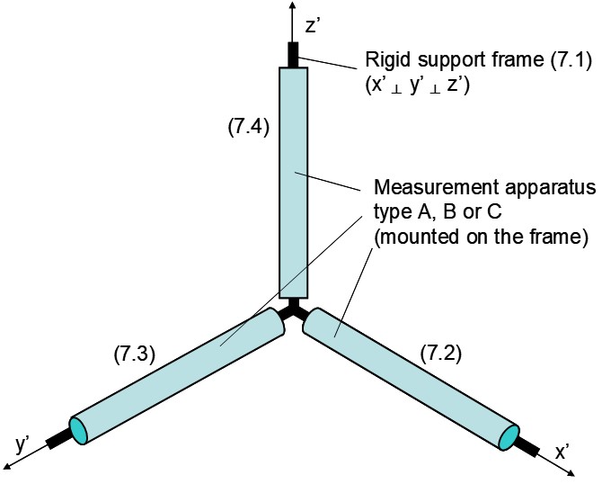
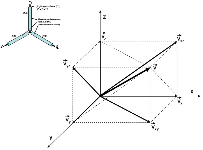
When having a three-dimensional set-up, as illustrated schematically in Figure 13, with three of such tube-shaped devices (each one according to Figure 33) perpendicular to one another, a full three-dimensional measurement system could be obtained. Such a set-up thus would enable to measure all real velocity vector components vx, vy and vz (thus in fact also the trajectory direction, Figure 14) in real space. If the signal shifts for all three measuring devices would be zero, the real velocity vector components vx, vy and vz thus would also be zero and such would indicate that the device is at perfect rest in real space in all directions. The basics of a three dimensional vector analysis of a velocity vector (v) of an object moving in real space is illustrated in Figure 14. In the three dimensional analysis in Figure 14, a velocity vectro v shows three vector components vx, vy and vz.
Only the two-dimensional case (x,y) will be discussed somewhat in this section since the reasoning for a three-dimensional case including (x,z) and (y,z) is analogous.
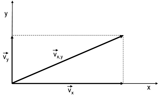
When having the two-dimensional situation as depicted in Figure 15 with a velocity vector (component) vxy in the plane (x,y), the RVMD will also move in the y-direction. From the fact that a photon being emitted in the direction perpendicular to the x-axis is “locked to real space” in its emission trajectory direction perpendicular to the x-axis it can be demonstrated that for the RVMD set-up of Figure 33 the measurement of vx is not influenced by the vy component of the velocity vector (as a result of the presence of the mirror and the forth and back trajectory traveling time of the photons being independent from the value of vy). It is not the intention of this website to make the complete analysis regarding all signal shift aspects within the three dimensional measuring set-up but the basics of the approach are already indicated here from such considerations.
It thus can be concluded that the real velocity vector of an object, which moves at a high velocity in real space, indeed can be measured on the basis of the trajectory of photons in real space since those photons are “locked to real space” and thus can be used as a “witness” (reference) of real space. A three dimensional RVMD can be mounted on a space ship or used on our planet to measure the complete real velocity vector without the need of an independent second material object “at rest” as a reference. In a space ship the RVMD would enable to read the real velocity, even in a confined compartment without any visual or whatever other contact with a second material object, considered to be “at rest”, from a relative point of view. A measuring concept and device is therefore possible which fully falsify the relativity paradigms by Galileo, Mach and others.
4.2 Determining an object’s real position from the perceived position by using the RVMD
It is common knowledge that the sun’s image arrives only on earth after 480 seconds since photons need that long time interval to travel the distance between the Sun and our planet. This means that an observer on Earth perceives the Sun in a past location in space, which happened already 480 seconds in the past and therefore the Sun’s actual “now” real location is in fact not observed but a location in the past. A sunset, when being defined in a geometrical way as the Sun’s exact location disappearing behind the Earth’s horizon as a result of the rotation of the Earth, obviously happened in reality 8 minutes ago while the perceived image as observed by an observer is linked to observed photons from the Sun corresponding to an eight minutes old image of the Sun’s location. An observer thus does not observe the Sun in its actual real location but in an apparent location. The observer therefore needs to make a correction on the perceived apparent location to obtain the real location of the Sun.
What then about the information delaying effect from the extremely high but still finite speed of light on Earth itself during an observation by an observer of an object? It is indeed clear for an observer Obs2 on Earth that the finite value of the speed of light results in a very small but definite travelling time of a photon, emitted by an observed photon source (the observed object), which emits photons towards a photon observation device (a theodolite, binoculars, telescope, camera, the eyes itself of the human observer …). In addition, as illustrated in preceding sections on this website, the effect of the EOVV on the location of arrival of a photon was demonstrated to be very significant. The same photon traveling time interval effect is of course also true when an observer on earth observes a stationary object on earth at a given distance. The photons coming from the observed object, as the information carriers of the object’s location, also need a definite travelling time before reaching the photon observation device and/or eyes of the observer. The information which the observer thus receives from those incoming photons is consequently also delayed according to the travelling time, needed by the photons.
An observer on Earth thus even always observes an observed object in the past! This may again seem totally negligible to the CPBDs at their first glance in the same way as the CPBDs did and even still do regarding my straightforward laser experiment and my irrefutable experimental result revealed in Figure 2. CPBDs thus still neglect in an irrational way the importance of that fact and also erroneously still not account for the theoretical and practical importance/potential and consequences of that fact. That fact is indeed extremely important since any observer on our planet also travels through space at, at least, the very high EOVV. As a result, the delay of the incoming photon information, at the the photon observation device and/or the eyes of the observer, from the observed object in fact causes a significant, thus not negligible, effect with respect to the interpretation of the object’s real location.
At this moment, no one knows the exact scalar value of the real velocity vector of the Earth in real space. There is indeed no exact velocity vector addition analysis of the multiple cosmological velocity vectors such as the:
- rotational SSOVV (Solar System Orbit Velocity Vector) within our galaxy (Milky Way)
- linear MWVV (Milky Way Velocity Vector) of our galaxy
- GGVVs (Galaxies Groups Velocity Vectors)
- GCVVs (Galaxies Clusters Velocity Vectors)
- superimposed inter-rotational orbit velocity vectors
- etc.
Thus, moreover, to what extent would all those velocity vectors attenuate one another, with respect to the velocity vector addition of all these numerous and even unknown velocity vectors? It should be noted that a measurement with my three dimensional RVMD would however even solve that question of course.
The additional very complicated three dimensional situation of the observer on our globe (24 hours rotation of the Earth; inclined rotation axis; longitude and latitude of the location of the observer on Earth; seasonal time instance) also needs a profound mathematical analysis. Evidently, such a detailed analysis would require a time demanding project and a team of specialists. As a result, only an oversimplified representation is presented here in Figure 17 showing an observer and an object, both stationary on “earth”. It is also assumed here for now that the scalar value of the EOVV is about 30000 meters per second, as also indicated in the literature, roughly corresponds to its real velocity in space. Of course this assumption should only be accepted here for demonstration reasons since in an accurate analysis a full three dimensional RVMD measurement would need to be done at the location of the observer. The “Earth” in this oversimplified example is therefore restricted to two dimensions, showing a rotation in a 24 h counter clockwise mode. The “Earth” also is assumed to show a real velocity of 30 000 m/sec in the x-direction in this oversimplified example. Corresponding to time intervals of 6 hours, four succeeding positions of the observer (Obs2) and the object (Obj) are drawn. In this example the observer Obs2 and the object are stationary on earth while the distance between the observer and the object is 10 000 m.
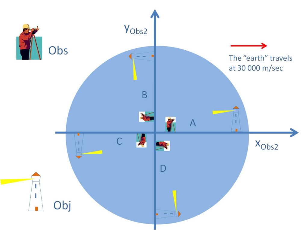
In the positions Obs2_B/Obj_B, the observer and the object move simultaneously in parallel in the positive x-direction. It clear that this resembles to the situation of the RVMD. A light signal departs from the object towards Obs2, in the y-direction. This situation is somewhat more complicated since it could be argued that a hypothetical single photon travelling perfectly in the y-direction could not be perceived by the observer since the observer also moves in the x-direction during the photon’s travelling time from the object to the observer. However, in real life, an object being illuminated by e.g. sunlight during daytime, is reflecting/scattering photons from each object’s surface point in all possible directions. Therefore it is clear that the photons which are actually visually captured by an observer’s eye are those photons which were send towards the observer at a particular (small) angle, a little off the y-direction. The trajectory could be analyzed in detail with the implementation of trigonometric formulas in order to exactly calculate that very small off-angle (trajectory in real space) and the marginally increased travelling distance and travelling time of the light signal towards the observer. For very large distances such exercise could be made but in this case, with the “small” distance of 10000 m between object and observer, it is assumed that the travelling time can be approximated well by the division of the distance of 10000 m by the speed of light, resulting in a travelling time of 3.335 x 10E-5 sec.
It can then be concluded that the difference between the object’s perceptible (image from the past object’s location; 3.335 x 10E-5 sec ago) and real position (now) is about 1 m since during the light signal travelling time of 3.335 x 10E-5 sec, the object has shifted that distance of 1 m in real space as a result of the high velocity of the Earth. The perceptible position of the object is thus estimated to be 1 m to the observer’s left (thus the real position is “+ 1 m” when compared to the perceived position). This estimate thus proves that it is very important in surveying applications, where light or a laser beam is used (photons as information carriers), to take into account the effect of the high velocity of our planet in space on the registered location of an object under survey. For an object at distances of 1000 m and 100 m these effects are estimated to be respectively 10 cm and 1 cm, to the left of the observer. That are extremely significant effects in surveying applications that CPBDs still have not taken into account, notwithstanding that I already made precise information available about these effects for over 15 years now (from 2006 through multiple private contacts, the internet, my website, etc.). Even more details can now be found in my Elsevier publication: Etienne Brauns, “On the concept and potential applications of a photons based device, measuring the velocity vector of an object, moving at high speed in space“, Results in Optics, 10 (2023) 100349, https://doi.org/10.1016/j.rio.2023.100349
For positions Obs2_D/Obj_D the difference between the object’s perceptible and real position is also about 1 m but in that case the perceptible position of the object is then 1 m further to the observer’s right (thus the real position is “- 1 m”). In the case of the positions Obs2_A/Obj_A and Obs2_C/Obj_C the difference between the object’s perceptible and real position in the example is estimated to be null to the left/righthand of the observer.
The situation in positions Obs2_B and Obs2_D involves a very small angular shift of 0.006° (which is about 0° 0’ 22”) which is not directly noticeable to the human eye. This angular shift is distant independent, in a way that a human’s visual perception is unable to detect the differences (luckily the speed of light is that high …). However, highly accurate measurement devices will detect the effect and this is clearly extremely important in a number of very high accuracy positioning (surveying) applications. Manufacturers of high end digital theodolites indeed claim an accuracy of 1 arcsec while the effect, as mentioned above, is 22 arcsec which is a factor of over 20 times larger than the claimed accuracy of 1 arcsec. It is thus obvious that in surveying application with such high end surveying measuring devices, which are based on angular measurements, corrections needs to be done in order to obtain accurate results. Such corrections could be done by the assistance of a three dimensional RVMD and by the calculation, through adequate transformation equations, of the real coordinates from the perceptible coordinates of the observed object. The extrapolation of the oversimplified one-dimensional based examples towards the real three-dimensional situation of the earth of course needs a much more complex analysis by experts in order to set up those correct transformation equations. In addition, the value of the real velocity needs to be measured first also. However, the example shows the basis of the approach which is needed for that matter.
Such effects thus cannot be neglected in high accuracy surveying applications such as e.g. large buildings or other large constructions (e.g. large span bridges when working simultaneously from both construction sides towards the middle of the construction). In a building application’s arbitrary example such as e.g. the Petronas twin towers in Kuala Lumpur with a height of about 500 m, a distance or height of 100 m involves a measuring device (surveying; theodolite) of which the reading then can show an “error” of -10 mm to + 10 mm with respect to the REAL position of the observed material object when compared to the PERCEIVED one. Moreover, such error is depending (alternating) from the rotational position of our planet (time instance of the measurement in a 24 h interval), longitude and latitude of the location of the measurement and the direction (east, west, north, south). Up to now, surveying measurement practice does not take into account these significant measurement error effects although they are thus extremely relevant and thus definitely should be accounted for.
It is therefore recommended to the Surveying Community to look into this all in a very detailed manner in order to then come to the needed conclusions regarding the urgently needed optimization of surveying protocols when using high end digital theodolites. Evidently a high end theodolite itself, showing an accuracy of 1 arcsec should also be able to detect the effect by simply measuring the coordinates of a fixed reference point at a wall (preferably in a temperature conditioned research room) while using a high end fixed theodolite at a distance of e.g. 10 m and then register through automated and continuous/ undisturbed time-lapse digital photography the theodolite 1 sec claimed arcsec accurate angle measurement changes linked to the survey of the fixed point at the wall over a period of 24 hour (by e.g. a digital data acquisition and registration each 15 minutes). The Lissajous effect shown in Figure 2 should then also be reflected in those theodolite measurement results and then will also confirm my findings. The theodolite will indeed register during the 24 hour test a change in the apparent angular coordinates of the fixed reference point (at the arcsec level). The change is caused by the fact that the photons being send from the reference point need time to arrive at the theodolite and thus are from the past. Since the angle between
- the direction defined by the theodolite and the reference point
- the direction of the velocity vector of our planet
changes in the same way, as in the laser example in Figure 2, it is clear that the change of the order of 20 arcsec should also be detected in the high end digital theodolite measurement results. Evidently the test needs to be performed properly which e.g. requires a stable floor for the theodolite tripod, a sufficiently long stabilizing settling period of the theodolite tripod to rule out mechanical effects (creep), an automated computerized data acquisition in order not to disturb the tripod manually after the stabilizing period, etc.